---
title: "collapse and sf"
subtitle: "Fast Manipulation of Simple Features Data Frames"
author: "Sebastian Krantz and Grant McDermott"
date: "2024-04-19"
output: 
  rmarkdown::html_vignette:
    toc: true

vignette: >
  %\VignetteIndexEntry{collapse and sf}
  %\VignetteEngine{knitr::rmarkdown}
  %\VignetteEncoding{UTF-8}
---

<style type="text/css">
pre {
  max-height: 900px;
  overflow-y: auto;
}

pre[class] {
  max-height: 900px;
}
</style>


<!--
*collapse* is a C/C++ based package for data transformation and statistical computing in R. It's aims are:

1. To facilitate complex data transformation, exploration and computing tasks in R.
2. To help make R code fast, flexible, parsimonious and programmer friendly. 
-->
This short vignette focuses on using *collapse* with the popular *sf* package by Edzer Pebesma. It shows that *collapse* supports easy manipulation of *sf* data frames, at computation speeds far above *dplyr*.

*collapse* v1.6.0 added internal support for *sf* data frames by having most essential functions (e.g., `fselect/gv`, `fsubset/ss`, `fgroup_by`, `findex_by`, `qsu`, `descr`, `varying`, `funique`, `roworder`, `rsplit`, `fcompute`, ...) internally handle the geometry column. 

To demonstrate this, we can load a test dataset provided by *sf*:


```r
library(collapse)
library(sf)

nc <- st_read(system.file("shape/nc.shp", package = "sf"), quiet = TRUE)
options(sf_max_print = 3)
nc
# Simple feature collection with 100 features and 14 fields
# Geometry type: MULTIPOLYGON
# Dimension:     XY
# Bounding box:  xmin: -84.32385 ymin: 33.88199 xmax: -75.45698 ymax: 36.58965
# Geodetic CRS:  NAD27
# First 3 features:
#    AREA PERIMETER CNTY_ CNTY_ID      NAME  FIPS FIPSNO CRESS_ID BIR74 SID74 NWBIR74 BIR79 SID79
# 1 0.114     1.442  1825    1825      Ashe 37009  37009        5  1091     1      10  1364     0
# 2 0.061     1.231  1827    1827 Alleghany 37005  37005        3   487     0      10   542     3
# 3 0.143     1.630  1828    1828     Surry 37171  37171       86  3188     5     208  3616     6
#   NWBIR79                       geometry
# 1      19 MULTIPOLYGON (((-81.47276 3...
# 2      12 MULTIPOLYGON (((-81.23989 3...
# 3     260 MULTIPOLYGON (((-80.45634 3...
```

## Summarising sf Data Frames

Computing summary statistics on *sf* data frames automatically excludes the 'geometry' column:


```r
# Which columns have at least 2 non-missing distinct values
varying(nc) 
#      AREA PERIMETER     CNTY_   CNTY_ID      NAME      FIPS    FIPSNO  CRESS_ID     BIR74     SID74 
#      TRUE      TRUE      TRUE      TRUE      TRUE      TRUE      TRUE      TRUE      TRUE      TRUE 
#   NWBIR74     BIR79     SID79   NWBIR79 
#      TRUE      TRUE      TRUE      TRUE

# Quick summary stats
qsu(nc)
#              N     Mean         SD    Min    Max
# AREA       100   0.1263     0.0492  0.042  0.241
# PERIMETER  100    1.673     0.4823  0.999   3.64
# CNTY_      100  1985.96   106.5166   1825   2241
# CNTY_ID    100  1985.96   106.5166   1825   2241
# NAME       100        -          -      -      -
# FIPS       100        -          -      -      -
# FIPSNO     100    37100     58.023  37001  37199
# CRESS_ID   100     50.5    29.0115      1    100
# BIR74      100  3299.62  3848.1651    248  21588
# SID74      100     6.67     7.7812      0     44
# NWBIR74    100  1050.81  1432.9117      1   8027
# BIR79      100  4223.92  5179.4582    319  30757
# SID79      100     8.36     9.4319      0     57
# NWBIR79    100  1352.81  1975.9988      3  11631

# Detailed statistics description of each column
descr(nc)
# Dataset: nc, 14 Variables, N = 100
# ----------------------------------------------------------------------------------------------------
# AREA (numeric): 
# Statistics
#     N  Ndist  Mean    SD   Min   Max  Skew  Kurt
#   100     77  0.13  0.05  0.04  0.24  0.48   2.5
# Quantiles
#     1%    5%   10%   25%   50%   75%  90%   95%   99%
#   0.04  0.06  0.06  0.09  0.12  0.15  0.2  0.21  0.24
# ----------------------------------------------------------------------------------------------------
# PERIMETER (numeric): 
# Statistics
#     N  Ndist  Mean    SD  Min   Max  Skew  Kurt
#   100     96  1.67  0.48    1  3.64  1.48  5.95
# Quantiles
#   1%    5%   10%   25%   50%   75%  90%   95%  99%
#    1  1.09  1.19  1.32  1.61  1.86  2.2  2.72  3.2
# ----------------------------------------------------------------------------------------------------
# CNTY_ (numeric): 
# Statistics
#     N  Ndist     Mean      SD   Min   Max  Skew  Kurt
#   100    100  1985.96  106.52  1825  2241  0.26  2.32
# Quantiles
#        1%       5%     10%      25%   50%      75%   90%     95%      99%
#   1826.98  1832.95  1837.9  1902.25  1982  2067.25  2110  2156.3  2238.03
# ----------------------------------------------------------------------------------------------------
# CNTY_ID (numeric): 
# Statistics
#     N  Ndist     Mean      SD   Min   Max  Skew  Kurt
#   100    100  1985.96  106.52  1825  2241  0.26  2.32
# Quantiles
#        1%       5%     10%      25%   50%      75%   90%     95%      99%
#   1826.98  1832.95  1837.9  1902.25  1982  2067.25  2110  2156.3  2238.03
# ----------------------------------------------------------------------------------------------------
# NAME (character): 
# Statistics
#     N  Ndist
#   100    100
# Table
#                Freq  Perc
# Ashe              1     1
# Alleghany         1     1
# Surry             1     1
# Currituck         1     1
# Northampton       1     1
# Hertford          1     1
# Camden            1     1
# Gates             1     1
# Warren            1     1
# Stokes            1     1
# Caswell           1     1
# Rockingham        1     1
# Granville         1     1
# Person            1     1
# ... 86 Others    86    86
# 
# Summary of Table Frequencies
#    Min. 1st Qu.  Median    Mean 3rd Qu.    Max. 
#       1       1       1       1       1       1 
# ----------------------------------------------------------------------------------------------------
# FIPS (character): 
# Statistics
#     N  Ndist
#   100    100
# Table
#                Freq  Perc
# 37009             1     1
# 37005             1     1
# 37171             1     1
# 37053             1     1
# 37131             1     1
# 37091             1     1
# 37029             1     1
# 37073             1     1
# 37185             1     1
# 37169             1     1
# 37033             1     1
# 37157             1     1
# 37077             1     1
# 37145             1     1
# ... 86 Others    86    86
# 
# Summary of Table Frequencies
#    Min. 1st Qu.  Median    Mean 3rd Qu.    Max. 
#       1       1       1       1       1       1 
# ----------------------------------------------------------------------------------------------------
# FIPSNO (numeric): 
# Statistics
#     N  Ndist   Mean     SD    Min    Max  Skew  Kurt
#   100    100  37100  58.02  37001  37199    -0   1.8
# Quantiles
#         1%       5%      10%      25%    50%      75%      90%      95%       99%
#   37002.98  37010.9  37020.8  37050.5  37100  37149.5  37179.2  37189.1  37197.02
# ----------------------------------------------------------------------------------------------------
# CRESS_ID (integer): 
# Statistics
#     N  Ndist  Mean     SD  Min  Max  Skew  Kurt
#   100    100  50.5  29.01    1  100     0   1.8
# Quantiles
#     1%    5%   10%    25%   50%    75%   90%    95%    99%
#   1.99  5.95  10.9  25.75  50.5  75.25  90.1  95.05  99.01
# ----------------------------------------------------------------------------------------------------
# BIR74 (numeric): 
# Statistics
#     N  Ndist     Mean       SD  Min    Max  Skew   Kurt
#   100    100  3299.62  3848.17  248  21588  2.79  11.79
# Quantiles
#       1%      5%    10%   25%     50%   75%     90%    95%       99%
#   283.64  419.75  531.8  1077  2180.5  3936  6725.7  11193  20378.22
# ----------------------------------------------------------------------------------------------------
# SID74 (numeric): 
# Statistics
#     N  Ndist  Mean    SD  Min  Max  Skew   Kurt
#   100     23  6.67  7.78    0   44  2.44  10.28
# Quantiles
#   1%  5%  10%  25%  50%   75%   90%    95%    99%
#    0   0    0    2    4  8.25  15.1  18.25  38.06
# ----------------------------------------------------------------------------------------------------
# NWBIR74 (numeric): 
# Statistics
#     N  Ndist     Mean       SD  Min   Max  Skew   Kurt
#   100     93  1050.81  1432.91    1  8027  2.83  11.84
# Quantiles
#   1%    5%   10%  25%    50%     75%     90%     95%      99%
#    1  9.95  39.2  190  697.5  1168.5  2231.8  3942.9  7052.84
# ----------------------------------------------------------------------------------------------------
# BIR79 (numeric): 
# Statistics
#     N  Ndist     Mean       SD  Min    Max  Skew  Kurt
#   100    100  4223.92  5179.46  319  30757  2.99  13.1
# Quantiles
#       1%     5%    10%      25%   50%   75%   90%       95%       99%
#   349.69  539.3  675.7  1336.25  2636  4889  8313  14707.45  26413.87
# ----------------------------------------------------------------------------------------------------
# SID79 (numeric): 
# Statistics
#     N  Ndist  Mean    SD  Min  Max  Skew  Kurt
#   100     28  8.36  9.43    0   57  2.28  9.88
# Quantiles
#   1%  5%  10%  25%  50%    75%  90%  95%    99%
#    0   0    1    2    5  10.25   21   26  38.19
# ----------------------------------------------------------------------------------------------------
# NWBIR79 (numeric): 
# Statistics
#     N  Ndist     Mean    SD  Min    Max  Skew   Kurt
#   100     98  1352.81  1976    3  11631  3.18  14.45
# Quantiles
#     1%    5%   10%    25%    50%      75%     90%     95%       99%
#   3.99  11.9  44.7  250.5  874.5  1406.75  2987.9  5090.5  10624.17
# ----------------------------------------------------------------------------------------------------
```


## Selecting Columns and Subsetting

We can select columns from the *sf* data frame without having to worry about taking along 'geometry':


```r
# Selecting a sequence of columns
fselect(nc, AREA, NAME:FIPSNO)
# Simple feature collection with 100 features and 4 fields
# Geometry type: MULTIPOLYGON
# Dimension:     XY
# Bounding box:  xmin: -84.32385 ymin: 33.88199 xmax: -75.45698 ymax: 36.58965
# Geodetic CRS:  NAD27
# First 3 features:
#    AREA      NAME  FIPS FIPSNO                       geometry
# 1 0.114      Ashe 37009  37009 MULTIPOLYGON (((-81.47276 3...
# 2 0.061 Alleghany 37005  37005 MULTIPOLYGON (((-81.23989 3...
# 3 0.143     Surry 37171  37171 MULTIPOLYGON (((-80.45634 3...

# Same using standard evaluation (gv is a shorthand for get_vars())
gv(nc, c("AREA", "NAME", "FIPS", "FIPSNO"))
# Simple feature collection with 100 features and 4 fields
# Geometry type: MULTIPOLYGON
# Dimension:     XY
# Bounding box:  xmin: -84.32385 ymin: 33.88199 xmax: -75.45698 ymax: 36.58965
# Geodetic CRS:  NAD27
# First 3 features:
#    AREA      NAME  FIPS FIPSNO                       geometry
# 1 0.114      Ashe 37009  37009 MULTIPOLYGON (((-81.47276 3...
# 2 0.061 Alleghany 37005  37005 MULTIPOLYGON (((-81.23989 3...
# 3 0.143     Surry 37171  37171 MULTIPOLYGON (((-80.45634 3...
```

The same applies to subsetting rows (and columns):


```r
# A fast and enhanced version of base::subset
fsubset(nc, AREA > fmean(AREA), AREA, NAME:FIPSNO)
# Simple feature collection with 44 features and 4 fields
# Geometry type: MULTIPOLYGON
# Dimension:     XY
# Bounding box:  xmin: -84.32385 ymin: 33.88199 xmax: -75.45698 ymax: 36.58965
# Geodetic CRS:  NAD27
# First 3 features:
#    AREA        NAME  FIPS FIPSNO                       geometry
# 1 0.143       Surry 37171  37171 MULTIPOLYGON (((-80.45634 3...
# 2 0.153 Northampton 37131  37131 MULTIPOLYGON (((-77.21767 3...
# 3 0.153  Rockingham 37157  37157 MULTIPOLYGON (((-79.53051 3...

# A fast version of `[` (where i is used and optionally j)
ss(nc, 1:10, c("AREA", "NAME", "FIPS", "FIPSNO"))
# Simple feature collection with 10 features and 4 fields
# Geometry type: MULTIPOLYGON
# Dimension:     XY
# Bounding box:  xmin: -84.32385 ymin: 33.88199 xmax: -75.45698 ymax: 36.58965
# Geodetic CRS:  NAD27
# First 3 features:
#    AREA      NAME  FIPS FIPSNO                       geometry
# 1 0.114      Ashe 37009  37009 MULTIPOLYGON (((-81.47276 3...
# 2 0.061 Alleghany 37005  37005 MULTIPOLYGON (((-81.23989 3...
# 3 0.143     Surry 37171  37171 MULTIPOLYGON (((-80.45634 3...
```

This is significantly faster than using `[`, `base::subset()`, `dplyr::select()` or `dplyr::filter()`: 


```r
library(microbenchmark)
library(dplyr)

# Selecting columns
microbenchmark(collapse = fselect(nc, AREA, NAME:FIPSNO), 
               dplyr = select(nc, AREA, NAME:FIPSNO),
               collapse2 = gv(nc, c("AREA", "NAME", "FIPS", "FIPSNO")), 
               sf = nc[c("AREA", "NAME", "FIPS", "FIPSNO")])
# Unit: microseconds
#       expr     min       lq      mean   median       uq      max neval
#   collapse   3.034   3.9565   5.19429   5.1865   5.6990   22.878   100
#      dplyr 431.279 452.2915 505.29015 466.3750 493.8450 3356.342   100
#  collapse2   2.665   3.4850   4.59610   4.4075   5.0635   14.391   100
#         sf 105.165 114.1235 120.39732 118.0390 124.9270  156.497   100
# Subsetting
microbenchmark(collapse = fsubset(nc, AREA > fmean(AREA), AREA, NAME:FIPSNO), 
               dplyr = select(nc, AREA, NAME:FIPSNO) |> filter(AREA > fmean(AREA)),
               collapse2 = ss(nc, 1:10, c("AREA", "NAME", "FIPS", "FIPSNO")), 
               sf = nc[1:10, c("AREA", "NAME", "FIPS", "FIPSNO")])
# Unit: microseconds
#       expr     min       lq       mean   median        uq      max neval
#   collapse   9.676  11.5825   15.01707  14.4730   16.8920   30.463   100
#      dplyr 890.643 917.6415 1055.40970 941.7085 1009.7890 5546.685   100
#  collapse2   2.829   3.5465    5.40585   4.8995    6.4165   20.541   100
#         sf 176.997 187.6160  202.72286 200.7565  210.8220  340.464   100
```

However, *collapse* functions don't subset the 'agr' attribute on selecting columns, which (if specified) relates columns (attributes) to the geometry, and also don't modify the 'bbox' attribute giving the overall boundaries of a set of geometries when subsetting the *sf* data frame. Keeping the full 'agr' attribute is not problematic for all practical purposes, but not changing 'bbox' upon subsetting may lead to too large margins when plotting the geometries of a subset *sf* data frame. 

One way to to change this is calling `st_make_valid()` on the subset frame; but `st_make_valid()` is very expensive, thus unless the subset frame is very small, it is better to use `[`, `base::subset()` or `dplyr::filter()` in cases where the bounding box size matters. 

## Aggregation and Grouping

The flexibility and speed of `collap()` for aggregation can be used on *sf* data frames. A separate method for *sf* objects was not considered necessary as one can simply aggregate the geometry column using `st_union()`:


```r
# Aggregating by variable SID74 using the median for numeric and the mode for categorical columns
collap(nc, ~ SID74, custom = list(fmedian = is.numeric, 
                                  fmode = is.character, 
                                  st_union = "geometry")) # or use is.list to fetch the geometry
# Simple feature collection with 23 features and 15 fields
# Geometry type: MULTIPOLYGON
# Dimension:     XY
# Bounding box:  xmin: -84.32385 ymin: 33.88199 xmax: -75.45698 ymax: 36.58965
# Geodetic CRS:  NAD27
# First 3 features:
#     AREA PERIMETER  CNTY_ CNTY_ID      NAME  FIPS FIPSNO CRESS_ID BIR74 SID74 SID74 NWBIR74  BIR79
# 1 0.0780    1.3070 1950.0  1950.0 Alleghany 37005  37073     37.0   487     0     0    40.0  594.0
# 2 0.0810    1.2880 1887.0  1887.0      Ashe 37009  37137     69.0   751     1     1   148.0  899.0
# 3 0.1225    1.6435 1959.5  1959.5   Caswell 37033  37078     39.5  1271     2     2   382.5 1676.5
#   SID79 NWBIR79                       geometry
# 1     1      45 MULTIPOLYGON (((-83.69563 3...
# 2     1     176 MULTIPOLYGON (((-80.02406 3...
# 3     2     452 MULTIPOLYGON (((-77.16129 3...
```

*sf* data frames can also be grouped and then aggregated using `fsummarise()`:


```r
nc |> fgroup_by(SID74)
# Simple feature collection with 100 features and 14 fields
# Geometry type: MULTIPOLYGON
# Dimension:     XY
# Bounding box:  xmin: -84.32385 ymin: 33.88199 xmax: -75.45698 ymax: 36.58965
# Geodetic CRS:  NAD27
# First 3 features:
#    AREA PERIMETER CNTY_ CNTY_ID      NAME  FIPS FIPSNO CRESS_ID BIR74 SID74 NWBIR74 BIR79 SID79
# 1 0.114     1.442  1825    1825      Ashe 37009  37009        5  1091     1      10  1364     0
# 2 0.061     1.231  1827    1827 Alleghany 37005  37005        3   487     0      10   542     3
# 3 0.143     1.630  1828    1828     Surry 37171  37171       86  3188     5     208  3616     6
#   NWBIR79                       geometry
# 1      19 MULTIPOLYGON (((-81.47276 3...
# 2      12 MULTIPOLYGON (((-81.23989 3...
# 3     260 MULTIPOLYGON (((-80.45634 3...
# 
# Grouped by:  SID74  [23 | 4 (4) 1-13]

nc |> 
  fgroup_by(SID74) |>
  fsummarise(AREA_Ag = fsum(AREA), 
             Perimeter_Ag = fmedian(PERIMETER),
             geometry = st_union(geometry))
# Simple feature collection with 23 features and 3 fields
# Geometry type: MULTIPOLYGON
# Dimension:     XY
# Bounding box:  xmin: -84.32385 ymin: 33.88199 xmax: -75.45698 ymax: 36.58965
# Geodetic CRS:  NAD27
# First 3 features:
#   SID74 AREA_Ag Perimeter_Ag                       geometry
# 1     0   1.103       1.3070 MULTIPOLYGON (((-83.69563 3...
# 2     1   0.914       1.2880 MULTIPOLYGON (((-80.02406 3...
# 3     2   1.047       1.6435 MULTIPOLYGON (((-77.16129 3...
```

Typically most of the time in aggregation is consumed by `st_union()` so that the speed of *collapse* does not really become visible on most datasets. A faster alternative is to use *geos* (*sf* backend for planar geometries) or *s2* (*sf* backend for spherical geometries) directly:


```r
# Using s2 backend: sensible for larger tasks
nc |> 
  fmutate(geometry = s2::as_s2_geography(geometry)) |>
  fgroup_by(SID74) |>
  fsummarise(AREA_Ag = fsum(AREA), 
             Perimeter_Ag = fmedian(PERIMETER),
             geometry = s2::s2_union_agg(geometry)) |>
  fmutate(geometry = st_as_sfc(geometry))
# Simple feature collection with 23 features and 3 fields
# Geometry type: MULTIPOLYGON
# Dimension:     XY
# Bounding box:  xmin: -84.32385 ymin: 33.88199 xmax: -75.45698 ymax: 36.58965
# Geodetic CRS:  WGS 84
# First 3 features:
#   SID74 AREA_Ag Perimeter_Ag                       geometry
# 1     0   1.103       1.3070 MULTIPOLYGON (((-83.69563 3...
# 2     1   0.914       1.2880 MULTIPOLYGON (((-80.02406 3...
# 3     2   1.047       1.6435 MULTIPOLYGON (((-77.16129 3...
```

In general, also upon aggregation with *collapse*, functions `st_as_sfc()`, `st_as_sf()`, or, in the worst case, `st_make_valid()`, may need to be invoked to ensure valid *sf* object output. Functions `collap()` and `fsummarise()` are attribute preserving but do not give special regard to geometry columns. 

One exception that both avoids the high cost of spatial functions in aggregation and any need for ex-post conversion/validation is aggregating spatial panel data over the time-dimension. Such panels can quickly be aggregated using `ffirst()` or `flast()` to aggregate the geometry:


```r
# Creating a panel-dataset by simply duplicating nc for 2 different years
pnc <- rowbind(`2000` = nc, `2001` = nc, idcol = "Year") |> as_integer_factor()
pnc 
# Simple feature collection with 200 features and 15 fields
# Geometry type: MULTIPOLYGON
# Dimension:     XY
# Bounding box:  xmin: -84.32385 ymin: 33.88199 xmax: -75.45698 ymax: 36.58965
# Geodetic CRS:  NAD27
# First 3 features:
#   Year  AREA PERIMETER CNTY_ CNTY_ID      NAME  FIPS FIPSNO CRESS_ID BIR74 SID74 NWBIR74 BIR79
# 1 2000 0.114     1.442  1825    1825      Ashe 37009  37009        5  1091     1      10  1364
# 2 2000 0.061     1.231  1827    1827 Alleghany 37005  37005        3   487     0      10   542
# 3 2000 0.143     1.630  1828    1828     Surry 37171  37171       86  3188     5     208  3616
#   SID79 NWBIR79                       geometry
# 1     0      19 MULTIPOLYGON (((-81.47276 3...
# 2     3      12 MULTIPOLYGON (((-81.23989 3...
# 3     6     260 MULTIPOLYGON (((-80.45634 3...

# Aggregating by NAME, using the last value for all categorical data
collap(pnc, ~ NAME, fmedian, catFUN = flast, cols = -1L)
# Simple feature collection with 100 features and 15 fields
# Geometry type: MULTIPOLYGON
# Dimension:     XY
# Bounding box:  xmin: -84.32385 ymin: 33.88199 xmax: -75.45698 ymax: 36.58965
# Geodetic CRS:  NAD27
# First 3 features:
#    AREA PERIMETER CNTY_ CNTY_ID      NAME      NAME  FIPS FIPSNO CRESS_ID BIR74 SID74 NWBIR74 BIR79
# 1 0.111     1.392  1904    1904  Alamance  Alamance 37001  37001        1  4672    13    1243  5767
# 2 0.066     1.070  1950    1950 Alexander Alexander 37003  37003        2  1333     0     128  1683
# 3 0.061     1.231  1827    1827 Alleghany Alleghany 37005  37005        3   487     0      10   542
#   SID79 NWBIR79                       geometry
# 1    11    1397 MULTIPOLYGON (((-79.24619 3...
# 2     2     150 MULTIPOLYGON (((-81.10889 3...
# 3     3      12 MULTIPOLYGON (((-81.23989 3...

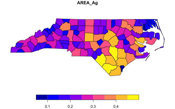
# Using fsummarise to aggregate just two variables and the geometry
pnc_ag <- pnc |> 
  fgroup_by(NAME) |>
  fsummarise(AREA_Ag = fsum(AREA), 
             Perimeter_Ag = fmedian(PERIMETER),
             geometry = flast(geometry))

# The geometry is still valid... (slt = shorthand for fselect)
plot(slt(pnc_ag, AREA_Ag))
```

<div class="figure">
<img src="https://raw.githubusercontent.com/SebKrantz/collapse/master/vignettes/figure/AREA_Ag-1.png" alt="plot of chunk AREA_Ag" width="100%" />
</div>

## Indexing

*sf* data frames can also become [*indexed frames*](https://sebkrantz.github.io/collapse/reference/indexing.html) (spatio-temporal panels):


```r
pnc <- pnc |> findex_by(CNTY_ID, Year)
pnc 
# Simple feature collection with 200 features and 15 fields
# Geometry type: MULTIPOLYGON
# Dimension:     XY
# Bounding box:  xmin: -84.32385 ymin: 33.88199 xmax: -75.45698 ymax: 36.58965
# Geodetic CRS:  NAD27
# First 3 features:
#   Year  AREA PERIMETER CNTY_ CNTY_ID      NAME  FIPS FIPSNO CRESS_ID BIR74 SID74 NWBIR74 BIR79
# 1 2000 0.114     1.442  1825    1825      Ashe 37009  37009        5  1091     1      10  1364
# 2 2000 0.061     1.231  1827    1827 Alleghany 37005  37005        3   487     0      10   542
# 3 2000 0.143     1.630  1828    1828     Surry 37171  37171       86  3188     5     208  3616
#   SID79 NWBIR79                       geometry
# 1     0      19 MULTIPOLYGON (((-81.47276 3...
# 2     3      12 MULTIPOLYGON (((-81.23989 3...
# 3     6     260 MULTIPOLYGON (((-80.45634 3...
# 
# Indexed by:  CNTY_ID [100] | Year [2]
qsu(pnc$AREA)
#          N/T    Mean      SD     Min     Max
# Overall  200  0.1263  0.0491   0.042   0.241
# Between  100  0.1263  0.0492   0.042   0.241
# Within     2  0.1263       0  0.1263  0.1263
settransform(pnc, AREA_diff = fdiff(AREA)) 
psmat(pnc$AREA_diff) |> head()
#      2000 2001
# 1825   NA    0
# 1827   NA    0
# 1828   NA    0
# 1831   NA    0
# 1832   NA    0
# 1833   NA    0
pnc <- unindex(pnc)
```

## Unique Values, Ordering, Splitting, Binding

Functions `funique()` and `roworder[v]()` ignore the 'geometry' column in determining the unique values / order of rows when applied to *sf* data frames. `rsplit()` can be used to (recursively) split an *sf* data frame into multiple chunks. 


```r
# Splitting by SID74
rsplit(nc, ~ SID74) |> head(2)
# $`0`
# Simple feature collection with 13 features and 13 fields
# Geometry type: MULTIPOLYGON
# Dimension:     XY
# Bounding box:  xmin: -84.32385 ymin: 33.88199 xmax: -75.45698 ymax: 36.58965
# Geodetic CRS:  NAD27
# First 3 features:
#    AREA PERIMETER CNTY_ CNTY_ID      NAME  FIPS FIPSNO CRESS_ID BIR74 NWBIR74 BIR79 SID79 NWBIR79
# 1 0.061     1.231  1827    1827 Alleghany 37005  37005        3   487      10   542     3      12
# 2 0.062     1.547  1834    1834    Camden 37029  37029       15   286     115   350     2     139
# 3 0.091     1.284  1835    1835     Gates 37073  37073       37   420     254   594     2     371
#                         geometry
# 1 MULTIPOLYGON (((-81.23989 3...
# 2 MULTIPOLYGON (((-76.00897 3...
# 3 MULTIPOLYGON (((-76.56251 3...
# 
# $`1`
# Simple feature collection with 11 features and 13 fields
# Geometry type: MULTIPOLYGON
# Dimension:     XY
# Bounding box:  xmin: -84.32385 ymin: 33.88199 xmax: -75.45698 ymax: 36.58965
# Geodetic CRS:  NAD27
# First 3 features:
#    AREA PERIMETER CNTY_ CNTY_ID      NAME  FIPS FIPSNO CRESS_ID BIR74 NWBIR74 BIR79 SID79 NWBIR79
# 1 0.114     1.442  1825    1825      Ashe 37009  37009        5  1091      10  1364     0      19
# 2 0.070     2.968  1831    1831 Currituck 37053  37053       27   508     123   830     2     145
# 3 0.124     1.428  1837    1837    Stokes 37169  37169       85  1612     160  2038     5     176
#                         geometry
# 1 MULTIPOLYGON (((-81.47276 3...
# 2 MULTIPOLYGON (((-76.00897 3...
# 3 MULTIPOLYGON (((-80.02567 3...
```

The default in `rsplit()` for data frames is `simplify = TRUE`, which, for a single LHS variable, would just split the column-vector. This does not apply to *sf* data frames as the 'geometry' column is always selected as well.


```r
# Only splitting Area
rsplit(nc, AREA ~ SID74) |> head(1)
# $`0`
# Simple feature collection with 13 features and 1 field
# Geometry type: MULTIPOLYGON
# Dimension:     XY
# Bounding box:  xmin: -84.32385 ymin: 33.88199 xmax: -75.45698 ymax: 36.58965
# Geodetic CRS:  NAD27
# First 3 features:
#    AREA                       geometry
# 1 0.061 MULTIPOLYGON (((-81.23989 3...
# 2 0.062 MULTIPOLYGON (((-76.00897 3...
# 3 0.091 MULTIPOLYGON (((-76.56251 3...

# For data frames the default simplify = TRUE drops the data frame structure
rsplit(qDF(nc), AREA ~ SID74) |> head(1)
# $`0`
#  [1] 0.061 0.062 0.091 0.064 0.059 0.080 0.066 0.099 0.094 0.078 0.131 0.167 0.051
```

*sf* data frames can be combined using `rowbind()`, which, by default, preserves the attributes of the first object.


```r
# Splitting by each row and recombining
nc_combined <- nc %>% rsplit(seq_row(.)) %>% rowbind() 
identical(nc, nc_combined)
# [1] TRUE
```

## Transformations

For transforming and computing columns, `fmutate()` and `ftransform[v]()` apply as to any other data frame. 

```r
fmutate(nc, gsum_AREA = fsum(AREA, SID74, TRA = "fill")) |> head()
# Simple feature collection with 6 features and 15 fields
# Geometry type: MULTIPOLYGON
# Dimension:     XY
# Bounding box:  xmin: -81.74107 ymin: 36.07282 xmax: -75.77316 ymax: 36.58965
# Geodetic CRS:  NAD27
# First 3 features:
#    AREA PERIMETER CNTY_ CNTY_ID      NAME  FIPS FIPSNO CRESS_ID BIR74 SID74 NWBIR74 BIR79 SID79
# 1 0.114     1.442  1825    1825      Ashe 37009  37009        5  1091     1      10  1364     0
# 2 0.061     1.231  1827    1827 Alleghany 37005  37005        3   487     0      10   542     3
# 3 0.143     1.630  1828    1828     Surry 37171  37171       86  3188     5     208  3616     6
#   NWBIR79                       geometry gsum_AREA
# 1      19 MULTIPOLYGON (((-81.47276 3...     0.914
# 2      12 MULTIPOLYGON (((-81.23989 3...     1.103
# 3     260 MULTIPOLYGON (((-80.45634 3...     1.380

# Same thing, more expensive
nc |> fgroup_by(SID74) |> fmutate(gsum_AREA = fsum(AREA)) |> fungroup() |> head()
# Simple feature collection with 6 features and 15 fields
# Geometry type: MULTIPOLYGON
# Dimension:     XY
# Bounding box:  xmin: -81.74107 ymin: 36.07282 xmax: -75.77316 ymax: 36.58965
# Geodetic CRS:  NAD27
# First 3 features:
#    AREA PERIMETER CNTY_ CNTY_ID      NAME  FIPS FIPSNO CRESS_ID BIR74 SID74 NWBIR74 BIR79 SID79
# 1 0.114     1.442  1825    1825      Ashe 37009  37009        5  1091     1      10  1364     0
# 2 0.061     1.231  1827    1827 Alleghany 37005  37005        3   487     0      10   542     3
# 3 0.143     1.630  1828    1828     Surry 37171  37171       86  3188     5     208  3616     6
#   NWBIR79                       geometry gsum_AREA
# 1      19 MULTIPOLYGON (((-81.47276 3...     0.914
# 2      12 MULTIPOLYGON (((-81.23989 3...     1.103
# 3     260 MULTIPOLYGON (((-80.45634 3...     1.380
```

Special attention to *sf* data frames is afforded by `fcompute()`, which can be used to compute new columns dropping existing ones - except for the geometry column and any columns selected through the `keep` argument. 


```r
fcompute(nc, scaled_AREA = fscale(AREA), 
             gsum_AREA = fsum(AREA, SID74, TRA = "fill"), 
         keep = .c(AREA, SID74))
# Simple feature collection with 100 features and 4 fields
# Geometry type: MULTIPOLYGON
# Dimension:     XY
# Bounding box:  xmin: -84.32385 ymin: 33.88199 xmax: -75.45698 ymax: 36.58965
# Geodetic CRS:  NAD27
# First 3 features:
#    AREA SID74 scaled_AREA gsum_AREA                       geometry
# 1 0.114     1  -0.2491860     0.914 MULTIPOLYGON (((-81.47276 3...
# 2 0.061     0  -1.3264176     1.103 MULTIPOLYGON (((-81.23989 3...
# 3 0.143     5   0.3402426     1.380 MULTIPOLYGON (((-80.45634 3...
```

## Conversion to and from *sf*

The quick converters `qDF()`, `qDT()`, and `qTBL()` can be used to efficiently convert *sf* data frames to standard data frames, *data.table*'s or *tibbles*, and the result can be converted back to the original *sf* data frame using `setAttrib()`, `copyAttrib()` or `copyMostAttrib()`. 


```r
library(data.table)
# Create a data.table on the fly to do an fast grouped rolling mean and back to sf
qDT(nc)[, list(roll_AREA = frollmean(AREA, 2), geometry), by = SID74] |> copyMostAttrib(nc)
# Simple feature collection with 100 features and 2 fields
# Geometry type: MULTIPOLYGON
# Dimension:     XY
# Bounding box:  xmin: -84.32385 ymin: 33.88199 xmax: -75.45698 ymax: 36.58965
# Geodetic CRS:  NAD27
# First 3 features:
#   SID74 roll_AREA                       geometry
# 1     1        NA MULTIPOLYGON (((-81.47276 3...
# 2     1     0.092 MULTIPOLYGON (((-76.00897 3...
# 3     1     0.097 MULTIPOLYGON (((-80.02567 3...
```

The easiest way to strip a geometry column off an *sf* data frame is via the function `atomic_elem()`, which removes list-like columns and, by default, also the class attribute. For example, we can create a *data.table* without list column using


```r
qDT(atomic_elem(nc)) |> head()
#     AREA PERIMETER CNTY_ CNTY_ID        NAME   FIPS FIPSNO CRESS_ID BIR74 SID74 NWBIR74 BIR79 SID79
#    <num>     <num> <num>   <num>      <char> <char>  <num>    <int> <num> <num>   <num> <num> <num>
# 1: 0.114     1.442  1825    1825        Ashe  37009  37009        5  1091     1      10  1364     0
# 2: 0.061     1.231  1827    1827   Alleghany  37005  37005        3   487     0      10   542     3
# 3: 0.143     1.630  1828    1828       Surry  37171  37171       86  3188     5     208  3616     6
# 4: 0.070     2.968  1831    1831   Currituck  37053  37053       27   508     1     123   830     2
# 5: 0.153     2.206  1832    1832 Northampton  37131  37131       66  1421     9    1066  1606     3
# 6: 0.097     1.670  1833    1833    Hertford  37091  37091       46  1452     7     954  1838     5
#    NWBIR79
#      <num>
# 1:      19
# 2:      12
# 3:     260
# 4:     145
# 5:    1197
# 6:    1237
```

This is also handy for other functions such as `join()` and `pivot()`, which are class agnostic like all of *collapse*, but do not have any built-in logic to deal with the *sf* column. 


```r
# Use atomic_elem() to strip geometry off y in left join
identical(nc, join(nc, atomic_elem(nc), overid = 2))
# left join: nc[AREA, PERIMETER, CNTY_, CNTY_ID, NAME, FIPS, FIPSNO, CRESS_ID, BIR74, SID74, NWBIR74, BIR79, SID79, NWBIR79] 100/100 (100%) <m:m> y[AREA, PERIMETER, CNTY_, CNTY_ID, NAME, FIPS, FIPSNO, CRESS_ID, BIR74, SID74, NWBIR74, BIR79, SID79, NWBIR79] 100/100 (100%)
# [1] TRUE

# In pivot: presently need to specify what to do with geometry column
pivot(nc, c("CNTY_ID", "geometry")) |> head()
# Simple feature collection with 6 features and 3 fields
# Geometry type: MULTIPOLYGON
# Dimension:     XY
# Bounding box:  xmin: -81.74107 ymin: 36.07282 xmax: -75.77316 ymax: 36.58965
# Geodetic CRS:  NAD27
# First 3 features:
#   CNTY_ID                       geometry variable value
# 1    1825 MULTIPOLYGON (((-81.47276 3...     AREA 0.114
# 2    1827 MULTIPOLYGON (((-81.23989 3...     AREA 0.061
# 3    1828 MULTIPOLYGON (((-80.45634 3...     AREA 0.143
# Or use
pivot(qDT(atomic_elem(nc)), "CNTY_ID") |> head()
#    CNTY_ID variable  value
#      <num>   <fctr> <char>
# 1:    1825     AREA  0.114
# 2:    1827     AREA  0.061
# 3:    1828     AREA  0.143
# 4:    1831     AREA   0.07
# 5:    1832     AREA  0.153
# 6:    1833     AREA  0.097
```

## Support for *units*

Since v2.0.13, *collapse* explicitly supports/preserves *units* objects through dedicated methods that preserve the 'units' class wherever sensible. 


```r
nc_dist <- st_centroid(nc) |> st_distance()
nc_dist[1:3, 1:3]
# Units: [m]
#          [,1]     [,2]     [,3]
# [1,]     0.00 34020.35 72728.02
# [2,] 34020.35     0.00 40259.55
# [3,] 72728.02 40259.55     0.00

fmean(nc_dist) |> head()
# Units: [m]
# [1] 250543.9 237040.0 217941.5 337016.5 250380.2 269604.6
fndistinct(nc_dist) |> head()
# [1] 100 100 100 100 100 100
```

## Conclusion

*collapse* provides no deep integration with the *sf* ecosystem and cannot perform spatial operations, but offers sufficient features and flexibility to painlessly manipulate *sf* data frames at much greater speeds than *dplyr*. 

This requires a bit of care by the user though to ensure that the returned *sf* objects are valid, especially following aggregation and subsetting.