iClusterVB

iClusterVB allows for fast integrative clustering and feature selection for high dimensional data.

Using a variational Bayes approach, its key features - clustering of mixed-type data, automated determination of the number of clusters, and feature selection in high-dimensional settings - address the limitations of traditional clustering methods while offering an alternative and potentially faster approach than MCMC algorithms, making iClusterVB a valuable tool for contemporary data analysis challenges.

Installation

You can install iClusterVB from CRAN with:

install.packages("iClusterVB")

You can install the development version of iClusterVB from GitHub with:

# install.packages("devtools")
devtools::install_github("AbdalkarimA/iClusterVB")

iClusterVB - The Main Function

Mandatory arguments

• mydata: A list of length R, where R is the number of datasets, containing the input data.

  • Note: For categorical data, 0’s must be re-coded to another, non-0 value.

• dist: A vector of length R specifying the type of data or distribution. Options include: “gaussian” (for continuous data), “multinomial” (for binary or categorical data), and “poisson” (for count data).

• K: The maximum number of clusters, with a default value of 10. The algorithm will converge to a model with dominant clusters, removing redundant clusters and automating the process of determining the number of clusters.

• initial_method: The method for the initial cluster allocation, which the iClusterVB algorithm will then use to determine the final cluster allocation. Options include “VarSelLCM” (default) for VarSelLCM, “random” for a random sample, “kproto” for k-prototypes, “kmeans” for k-means (continuous data only), “mclust” for mclust (continuous data only), or “lca” for poLCA (categorical data only).

• VS_method: The feature selection method. The options are 0 (default) for clustering without feature selection and 1 for clustering with feature selection

• initial_cluster: The initial cluster membership. The default is NULL, which uses initial_method for initial cluster allocation. If it is not NULL, it will overwrite the previous initial values setting for this parameter.

• initial_vs_prob: The initial feature selection probability, a scalar. The default is NULL, which assigns a value of 0.5.

• initial_fit: Initial values based on a previously fitted iClusterVB model (an iClusterVB object). The default is NULL.

• initial_omega: Customized initial values for feature inclusion probabilities. The default is NULL. If the argument is not NULL, it will overwrite the previous initial values setting for this parameter. If VS_method = 1, initial_omega is a list of length R, and each element of the list is an array with dim=c(N,p\[\[r\]])). N is the sample size and p\[\[r\]] is the number of features for dataset r, r = 1,…,R.

• initial_hyper_parameters: A list of the initial hyper-parameters of the prior distributions for the model. The default is NULL, which assigns alpha_00 = 0.001, mu_00 = 0,
s2_00 = 100, a_00 = 1, b_00 = 1, kappa_00 = 1, u_00 = 1, v_00 = 1. These are \(\pmb{\alpha}_0, \mu_0, s^2_0, a_0, b_0, \pmb{\kappa}_0, c_0, \text{and } d_0\) described in the research article that was submitted. The citation will be updated to display the paper once it is ready.

• max_iter: The maximum number of iterations for the VB algorithm. The default is 200.

• early_stop: Whether to stop the algorithm upon convergence or to continue until max_iter is reached. Options are 1 (default) to stop when the algorithm converges, and 0 to stop only when max_iter is reached.

• per: Print information every “per” iteration. The default is 10.

• convergence_threshold: The convergence threshold for the change in ELBO. The default is 0.0001.

Simulated Data

We will demonstrate the clustering and feature selection performance of iClusterVB using a simulated dataset comprising \(N = 240\) individuals and \(R = 4\) data views with different data types. Two views were continuous, one was count, and one was binary – a setup commonly found in genomics data where gene or mRNA expression (continuous), DNA copy number (count), and mutation presence (binary) are observed. The true number of clusters (\(K\)) was set to 4, with balanced cluster proportions (\(\pi_1 = 0.25, \pi_2 = 0.25, \pi_3 = 0.25, \pi_4 = 0.25\)). Each data view consisted of \(p_r = 500\) features (\(r = 1, \dots, 4\)), totaling \(p = \sum_{r=1}^4 p_r = 2000\) features across all views. Within each view, only 50 features (10%) were relevant for clustering, while the remaining features were noise. The relevant features were distributed across clusters as described in the table below:

The simulated dataset is included as a list in the package.

Data pre-processing

library(iClusterVB)

# Input data must be a list

dat1 <- list(gauss_1 = sim_data$continuous1_data,
             gauss_2 = sim_data$continuous2_data,
             multinomial_1 = sim_data$binary_data,
             poisson_1 = sim_data$count_data)

dist <- c("gaussian", "gaussian",
          "multinomial", "poisson")

# Re-code `0`s to `2`s. This must be done for feature selection 
# and clustering to work properly.
dat1$multinomial_1[dat1$multinomial_1 == 0] <- 2

Running the model

set.seed(123)
fit_iClusterVB <- iClusterVB(
  mydata = dat1,
  dist = dist,
  K = 8,
  initial_method = "VarSelLCM",
  VS_method = 1, # Variable Selection is on
  max_iter = 100,
  per = 100
)
#> ------------------------------------------------------------
#> Pre-processing and initializing the model
#> ------------------------------------------------------------
#> ------------------------------------------------------------
#> Running the CAVI algorithm
#> ------------------------------------------------------------
#> iteration = 100 elbo = -43591384.761314

Comparing to True Cluster Membership

table(fit_iClusterVB$cluster, sim_data$cluster_true)
#>    
#>      1  2  3  4
#>   2 60  0  0  0
#>   4  0 60  0  0
#>   6  0  0 60  0
#>   8  0  0  0 60

Summary of the Model

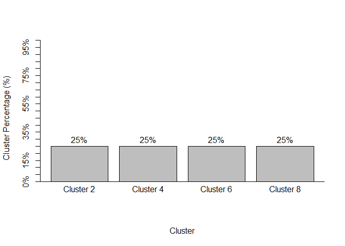
# We can obtain a summary using summary()
summary(fit_iClusterVB)
#> Total number of individuals:
#> [1] 240
#> 
#> User-inputted maximum number of clusters: 8
#> Number of clusters determined by algorithm: 4
#> 
#> Cluster Membership:
#>  2  4  6  8 
#> 60 60 60 60 
#> 
#> # of variables above the posterior inclusion probability of 0.5 for View 1 - gaussian
#> [1] "58 out of a total of 500"
#> 
#> # of variables above the posterior inclusion probability of 0.5 for View 2 - gaussian
#> [1] "59 out of a total of 500"
#> 
#> # of variables above the posterior inclusion probability of 0.5 for View 3 - multinomial
#> [1] "62 out of a total of 500"
#> 
#> # of variables above the posterior inclusion probability of 0.5 for View 4 - poisson
#> [1] "69 out of a total of 500"

Generic Plots

plot(fit_iClusterVB)

Probability of Inclusion Plots

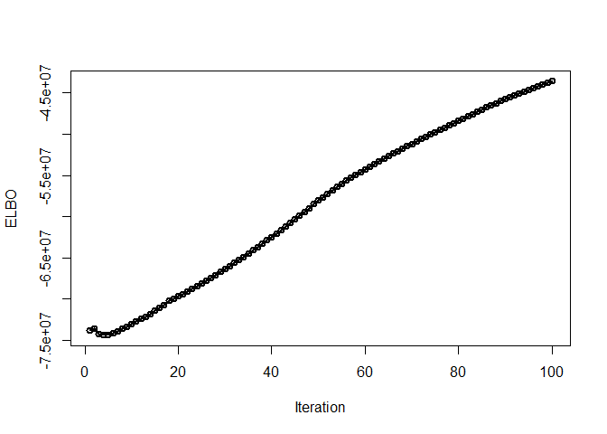
# The `piplot` function can be used to visualize the probability of inclusion

piplot(fit_iClusterVB)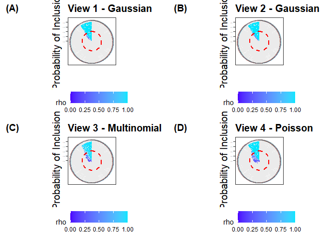

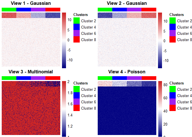
Heat maps to visualize the clusters

# The `chmap` function can be used to display heat maps for each data view

list_of_plots <- chmap(fit_iClusterVB, rho = 0,
      cols = c("green", "blue",
               "purple", "red"),
      scale = "none")

# The `grid.arrange` function from gridExtra can be used to display all the 
# plots together
gridExtra::grid.arrange(grobs = list_of_plots, ncol = 2, nrow = 2)