![]()
![]()
![]()
The gellipsoid package extends the class of geometric ellipsoids to
“generalized ellipsoids”, which allow degenerate ellipsoids that are
flat and/or unbounded. Thus, ellipsoids can be naturally defined to
include lines, hyperplanes, points, cylinders, etc. The methods can be
used to represent generalized ellipsoids in a -dimensional space
, with plots in up to 3D.
The goal is to be able to think about, visualize, and compute a
linear transformation of an ellipsoid with central matrix or its inverse
which apply equally to unbounded
and/or degenerate ellipsoids. This permits exploration of a variety to
statistical issues that can be visualized using ellipsoids as discussed
by Friendly, Fox & Monette (2013), Elliptical Insights:
Understanding Statistical Methods Through Elliptical Geometry doi:10.1214/12-STS402.
The implementation uses a representation, based on
the singular value decomposition (SVD) of an ellipsoid-generating
matrix,
, where
is square orthogonal and
is diagonal.
For the usual, “proper” ellipsoids, is positive-definite so all elements of
are positive. In generalized ellipsoids,
is extended to non-negative real numbers,
i.e. its elements can be 0, Inf or a positive real.
A proper ellipsoid in can be defined by
where
is a non-negative definite central matrix,
In applications,
is typically a variance-covariance matrix A
proper ellipsoid is bounded, with a non-empty interior. We call
these fat ellipsoids.
A degenerate flat ellipsoid corresponds to one where the
central matrix is singular or when there are one or more
zero singular values in
. In 3D, a generalized ellipsoid that is
flat in one dimension (
)
collapses to an ellipse; one that is flat in two dimensions (
)
collapses to a line, and one that is flat in three dimensions collapses
to a point.
An unbounded ellipsoid is one that has infinite extent in
one or more directions, and is characterized by infinite singular values
in . For example, in 3D, an unbounded ellipsoid
with one infinite singular value is an infinite cylinder of elliptical
cross-section.
gell() Constructs a generalized ellipsoid using the
representation. The
inputs can be specified in a variety of ways:
dual() calculates the dual or inverse of a
generalized ellipsoid
gmult() calculates a linear transformation of a
generalized ellipsoid
signature() calculates the signature of a
generalized ellipsoid, a vector of length 3 giving the number of
positive, zero and infinite singular values in the (U, D)
representation.
ell3d() Plots generalized ellipsoids in 3D using the
rgl package
You can install the development version of gellipsoid from GitHub with:
# install.packages("devtools")
devtools::install_github("friendly/gellipsoid")The following examples illustrate gell objects and their
properties. Each of these may be plotted in 3D using
ell3d(). These objects can be specified in a variety of
ways, but for these examples the span is simplest.
A unit sphere in has a central matrix of the identity
matrix.
library(gellipsoid)
(zsph <- gell(Sigma = diag(3)))  # a unit sphere in R^3
#> $center
#> [1] 0 0 0
#>
#> $u
#>      [,1] [,2] [,3]
#> [1,]    0    0    1
#> [2,]    0    1    0
#> [3,]    1    0    0
#>
#> $d
#> [1] 1 1 1
#>
#> attr(,"class")
#> [1] "gell"
signature(zsph)
#>  pos zero  inf
#>    3    0    0
isBounded(zsph)
#> [1] TRUE
isFlat(zsph)
#> [1] FALSE
A plane in is flat in one dimension.
(zplane <- gell(span = diag(3)[, 1:2]))  # a plane
#> $center
#> [1] 0 0 0
#>
#> $u
#>      [,1] [,2] [,3]
#> [1,]    1    0    0
#> [2,]    0    1    0
#> [3,]    0    0    1
#>
#> $d
#> [1] Inf Inf   0
#>
#> attr(,"class")
#> [1] "gell"
signature(zplane)
#>  pos zero  inf
#>    0    1    2
isBounded(zplane)
#> [1] FALSE
isFlat(zplane)
#> [1] TRUE

dual(zplane)  # line orthogonal to that plane
#> $center
#> [1] 0 0 0
#>
#> $u
#>      [,1] [,2] [,3]
#> [1,]    0    0    1
#> [2,]    0    1    0
#> [3,]    1    0    0
#>
#> $d
#> [1] Inf   0   0
#>
#> attr(,"class")
#> [1] "gell"
signature(dual(zplane))
#>  pos zero  inf
#>    0    2    1
A hyperplane. Note that the gell object with a center
contains more information than the geometric plane.
(zhplane <- gell(center = c(0, 0, 2),
                 span = diag(3)[, 1:2]))  # a hyperplane
#> $center
#> [1] 0 0 2
#>
#> $u
#>      [,1] [,2] [,3]
#> [1,]    1    0    0
#> [2,]    0    1    0
#> [3,]    0    0    1
#>
#> $d
#> [1] Inf Inf   0
#>
#> attr(,"class")
#> [1] "gell"
signature(zhplane)
#>  pos zero  inf
#>    0    1    2

dual(zhplane)  # orthogonal line through same center
#> $center
#> [1] 0 0 2
#>
#> $u
#>      [,1] [,2] [,3]
#> [1,]    0    0    1
#> [2,]    0    1    0
#> [3,]    1    0    0
#>
#> $d
#> [1] Inf   0   0
#>
#> attr(,"class")
#> [1] "gell"
A point:
zorigin <- gell(span = cbind(c(0, 0, 0)))
signature(zorigin)
#>  pos zero  inf
#>    0    3    0

# what is the dual (inverse) of a point?
dual(zorigin)
#> $center
#> [1] 0 0 0
#>
#> $u
#>      [,1] [,2] [,3]
#> [1,]    0    0    1
#> [2,]    0    1    0
#> [3,]    1    0    0
#>
#> $d
#> [1] Inf Inf Inf
#>
#> attr(,"class")
#> [1] "gell"

signature(dual(zorigin))
#>  pos zero  inf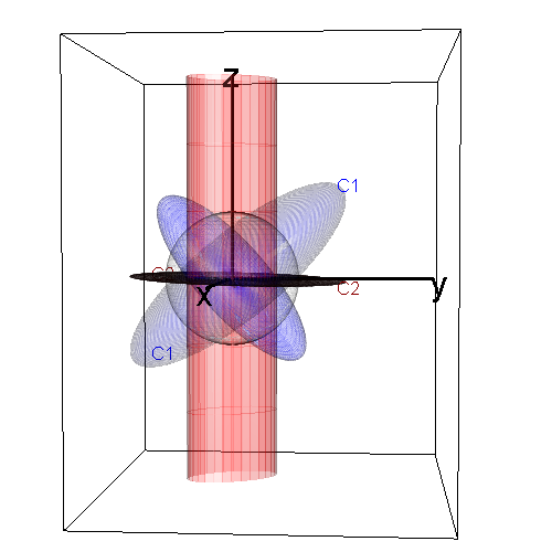
#> 0 0 3The following figure shows views of two generalized ellipsoids. (blue) determines a proper, fat ellipsoid; it’s inverse
also generates a proper ellipsoid.
(red) determines an improper, flat ellipsoid,
whose inverse
is an unbounded cylinder of
elliptical cross-section.
is the projection of
onto the plane where
. The scale of these ellipsoids is defined
by the gray unit sphere.
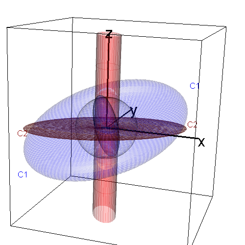
This figure illustrates the orthogonality of each and its dual,
.
Friendly, M., Monette, G. and Fox, J. (2013). Elliptical Insights: Understanding Statistical Methods through Elliptical Geometry. Online paper
Friendly, M. (2013). Supplementary materials for “Elliptical Insights …”, https://www.datavis.ca/papers/ellipses/