The PDXpower package can conduct power analysis for
time-to-event outcome based on empirical simulations.
You can install the development version of PDXpower from
GitHub with:
# install.packages("devtools")
devtools::install_github("shanpengli/PDXpower")Below is a toy example how to conduct power analysis based on a
preliminary dataset animals1. Particularly, we need to
specify a formula that fits a ANOVA mixed effects model with correlating
variables in animals1, where ID is the PDX
line number, Y is the event time variable, and
Tx is the treatment variable.
Next, run power analysis by fitting a ANOVA mixed effects model on
animals1.
library(PDXpower)
#> Loading required package: survival
#> Loading required package: parallel
data(animals1)
### Power analysis on a preliminary dataset by assuming the time to event is log-normal
PowTab <- PowANOVADat(data = animals1, formula = log(Y) ~ Tx,
                      random = ~ 1|ID, n = c(3, 5, 10), m = c(2, 3, 4), sim = 100)
#> Parameter estimates based on the pilot data:
#> Treatment effect (beta): 0.7299
#> Variance of random effect (tau2): 0.0332
#> Random error variance (sigma2): 0.386
#>
#> Monte Carlo power estimate, calculated as the
#>   proportion of instances where the null hypothesis
#>   H_0: beta = 0 is rejected (n = number of PDX lines,
#>   m = number of animals per arm per PDX line,
#>   N = total number of animals for a given combination of n and m):
#>    n m  N Power (%)
#> 1  3 2 12        43
#> 2  3 3 18        65
#> 3  3 4 24        77
#> 4  5 2 20        70
#> 5  5 3 30        87
#> 6  5 4 40        95
#> 7 10 2 40        98
#> 8 10 3 60        99
#> 9 10 4 80       100
The following code generates a power curve based on the object
PowTab.
plotpower(PowTab[[4]], ylim = c(0, 1))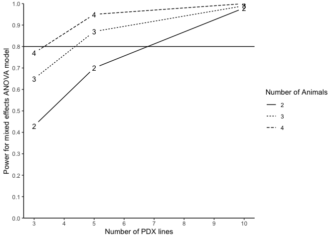
Or we can fit a ANOVA fixed effect model for running power analysis.
### Power analysis by specifying the median survival
### of control and treatment group and assuming
### the time-to-event is log-normal distributed
PowTab <- PowANOVA(ctl.med.surv = 2.4, tx.med.surv = 7.2, icc = 0.1, sigma2 = 1, sim = 100, n = c(3, 5, 10), m = c(2, 3, 4))
#> Treatment effect (beta): -1.098612
#> Variance of random effect (tau2): 0.1111111
#> Intra-PDX correlation coefficient (icc): 0.1
#> Random error variance (sigma2): 1
#>
#> Monte Carlo power estimate, calculated as the
#>   proportion of instances where the null hypothesis
#>   H_0: beta = 0 is rejected (n = number of PDX lines,
#>   m = number of animals per arm per PDX line,
#>   N = total number of animals for a given combination
#>   of n and m):
#>    n m  N Power (%)
#> 1  3 2 12        37
#> 2  3 3 18        56
#> 3  3 4 24        85
#> 4  5 2 20        65
#> 5  5 3 30        80
#> 6  5 4 40        97
#> 7 10 2 40        93
#> 8 10 3 60        99
#> 9 10 4 80       100
Alternatively, one can run power analysis by fitting a Cox frailty
model. Here we present another dataset animals2.
Particularly, we need to specify a formula that fits a Cox frailty model
with correlating variables in animals2, where
ID is the PDX line number, Y is the event time
variable, Tx is the treatment variable, and
status is the event status.
data(animals2)
### Power analysis on a preliminary dataset by assuming the time to event is Weibull-distributed
PowTab <- PowFrailtyDat(data = animals2, formula = Surv(Y, status) ~ Tx + cluster(ID),
                        n = c(3, 5, 10), m = c(2, 3, 4), sim = 100)
#> Parameter estimates based on the pilot data:
#> Scale parameter (lambda): 0.0154
#> Shape parameter (nu): 2.1722
#> Treatment effect (beta): -0.8794
#> Variance of random effect (tau2): 0.0422
#>
#> Monte Carlo power estimate, calculated as the
#>   proportion of instances where the null hypothesis
#>   H_0: beta = 0 is rejected (n = number of PDX lines,
#>   m = number of animals per arm per PDX line,
#>   N = total number of animals for a given combination
#>   of n and m,
#>   Censoring Rate = average censoring rate across 500
#>   Monte Carlo samples):
#>    n m  N Power (%) for Cox's frailty Censoring Rate
#> 1  3 2 12                       36.49              0
#> 2  3 3 18                       42.35              0
#> 3  3 4 24                       62.22              0
#> 4  5 2 20                       49.30              0
#> 5  5 3 30                       69.23              0
#> 6  5 4 40                       78.72              0
#> 7 10 2 40                       90.57              0
#> 8 10 3 60                       88.78              0
#> 9 10 4 80                       96.91              0
PowTab
#> $lambda
#> [1] 0.01540157
#>
#> $nu
#> [1] 2.172213
#>
#> $beta
#>        Tx
#> -0.879356
#>
#> $tau2
#> [1] 0.04224566
#>
#> $PowTab
#>    n m  N Power (%) for Cox's frailty Censoring Rate
#> 1  3 2 12                       36.49              0
#> 2  3 3 18                       42.35              0
#> 3  3 4 24                       62.22              0
#> 4  5 2 20                       49.30              0
#> 5  5 3 30                       69.23              0
#> 6  5 4 40                       78.72              0
#> 7 10 2 40                       90.57              0
#> 8 10 3 60                       88.78              0
#> 9 10 4 80                       96.91              0
#>
#> attr(,"class")
#> [1] "PowFrailtyDat"
The following code generates a power curve based on the object
PowTab.
plotpower(PowTab[[5]], ylim = c(0, 1))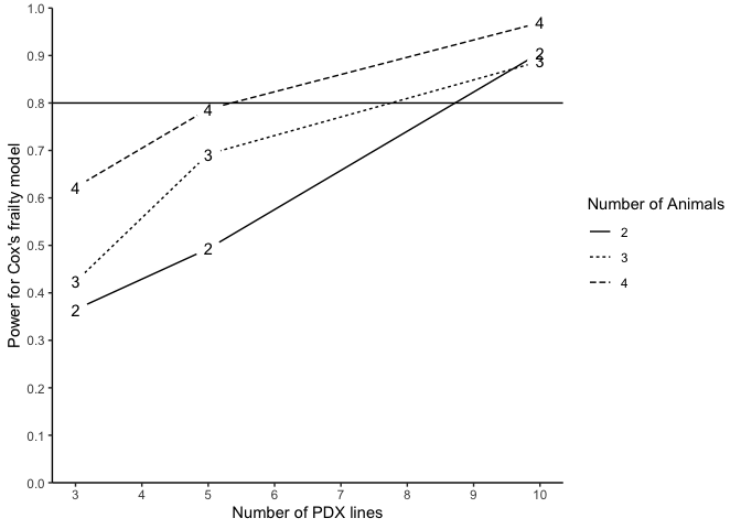
Alternatively, we may also conduct power analysis based on median
survival of two randomized arms. We suppose that the median survival of
the control and treatment arm is 2.4 and 4.8, allowing a PDX line has
10% marginal error (tau2=0.1) of treatment effect and an
exponential event time, a power analysis may be done as below:
### Assume the time to event outcome is weibull-distributed
PowTab <- PowFrailty(ctl.med.surv = 2.4, tx.med.surv = 4.8, nu = 1, tau2 = 0.1, sim = 100,
                     n = c(3, 5, 10), m = c(2, 3, 4))
#> Treatment effect (beta): -0.6931472
#> Scale parameter (lambda): 0.2888113
#> Shape parameter (nu): 1
#> Variance of random effect (tau2): 0.1
#>
#> Monte Carlo power estimate, calculated as the
#>   proportion of instances where the null hypothesis
#>   H_0: beta = 0 is rejected (n = number of PDX lines,
#>   m = number of animals per arm per PDX line,
#>   N = total number of animals for a given combination
#>   of n and m,
#>   Censoring Rate = average censoring rate across 500
#>   Monte Carlo samples):
#>    n m  N Power (%) for Cox's frailty Censoring Rate
#> 1  3 2 12                       22.45              0
#> 2  3 3 18                       21.05              0
#> 3  3 4 24                       41.41              0
#> 4  5 2 20                       35.16              0
#> 5  5 3 30                       44.79              0
#> 6  5 4 40                       62.89              0
#> 7 10 2 40                       67.01              0
#> 8 10 3 60                       73.74              0
#> 9 10 4 80                       86.73              0